Capítulo 8 Gráficos bivariados

dados <- read.table("data/iris.csv", dec = ",", header = TRUE)
str(dados)

## 'data.frame':    150 obs. of  5 variables:
##  $ Sepal.Length: num  5.1 4.9 4.7 4.6 5 5.4 4.6 5 4.4 4.9 ...
##  $ Sepal.Width : num  3.5 3 3.2 3.1 3.6 3.9 3.4 3.4 2.9 3.1 ...
##  $ Petal.Length: num  1.4 1.4 1.3 1.5 1.4 1.7 1.4 1.5 1.4 1.5 ...
##  $ Petal.Width : num  0.2 0.2 0.2 0.2 0.2 0.4 0.3 0.2 0.2 0.1 ...
##  $ Species     : Factor w/ 3 levels "setosa","versicolor",..: 1 1 1 1 1 1 1 1 1 1 ...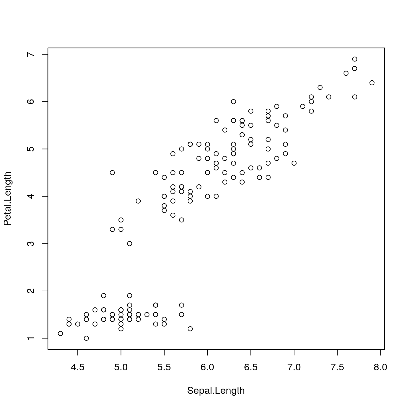

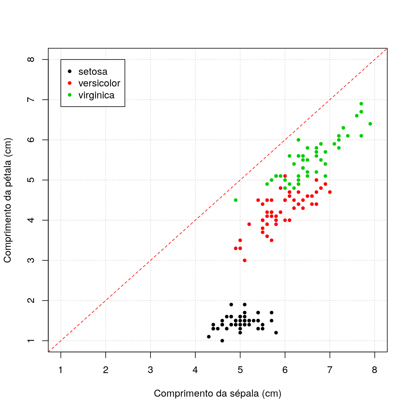
plot(dados[, c("Sepal.Length", "Petal.Length")])

plot(dados[, c("Sepal.Length", "Petal.Length")],
     xlab = "Comprimento da sépala (cm)",
     ylab = "Comprimento da pétala (cm)",
     xlim = c(1, 8), ylim = c(1, 8), pch = 20,
     panel.first = grid(), col = dados[, "Species"])
abline(a = 0, b = 1, col = "red", lty = "dashed")
legend(x = 1, y = 8, legend = levels(dados[, "Species"]), 
       col = 1:3, pch = 20, )